Method
This page describes how we construct interpretable steering directions from SAE latents. The method is structured as a five-stage pipeline; we walk through each stage in detail below.
Pipeline Overview
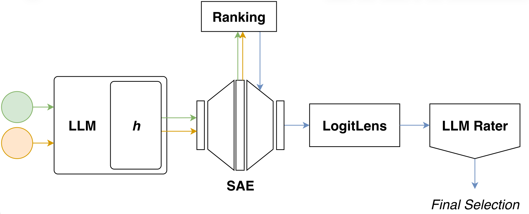
Our methodology comprises five sequential stages:
- Activation Extraction — obtain activation vectors from the base LLM at a specified layer using contrastive prompt sets.
- SAE Encoding — project these activations into the corresponding SAE latent space.
- Latent Ranking — score and select the top-$k$ candidate latents based on their SAE activation patterns.
- Logit Lens Projection — decode selected latents back to model dimensionality and identify their most promoted tokens.
- Semantic Validation — evaluate candidate latents through an LLM judge based on their token promotion profiles.
Pipeline Stages
Activation Extraction
The first stage extracts hidden state representations from the base language model using contrastive prompt sets. We provide the model with two sets of inputs: positive examples that exhibit the target concept or behavior, and negative examples that lack this property. For each set, we compute activations at a specified layer where we intend to apply the steering intervention.
Formally, given $P$ positive prompts ${p_i^+}_{i=1}^P$ and $N$ negative prompts ${p_i^-}_{i=1}^N$, we extract hidden state activations from the model’s residual stream at layer $\ell$, using the final token position throughout, as it contains the model’s aggregated representation of the entire input sequence. This yields two sets of $d_{\text{model}}$-dimensional activation vectors:
\[\begin{align} \mathcal{A}^+ &= \{a_\ell(p_i^+)\}_{i=1}^P \\ \mathcal{A}^- &= \{a_\ell(p_i^-)\}_{i=1}^N \end{align}\]where $a_\ell(p) \in \mathbb{R}^{d_{\text{model}}}$ denotes the activation at layer $\ell$ for the final token of prompt $p$. These contrastive activation sets serve as inputs for the subsequent SAE encoding stage.
SAE Encoding
Given $\mathcal{A}^+$ and $\mathcal{A}^-$, we pass them through the SAE encoder to obtain sparse representations in the SAE latent space:
\[\begin{align} \mathcal{Z}^+ &= \{\text{Enc}_{\text{SAE}}(a) \mid a \in \mathcal{A}^+\} \\ \mathcal{Z}^- &= \{\text{Enc}_{\text{SAE}}(a) \mid a \in \mathcal{A}^-\} \end{align}\]Each resulting latent vector $z \in \mathbb{R}^{d_{\text{SAE}}}$ provides a sparse decomposition of the original activation into SAE features. Although $z$ is high-dimensional, only a small subset of SAE latents is active for any given input $a$.
Latent Ranking
Our goal is to identify a small set of good SAE latents to serve as building blocks for the final steering direction. Given $\mathcal{Z}^+$ and $\mathcal{Z}^-$, we ask which latents appear most characteristic of the target concept and operationalize this via a family of ranking scores. How well each score finds semantically relevant latents, and whether the highest-ranked latents also yield better steering, is evaluated empirically in Results.
All ranking scores are built from two basic quantities:
- Frequency difference — how much more often a latent is active in the target set than in the contrastive set.
- Magnitude difference — how much stronger a latent activates in the target set when it is active.
For each latent $j$, let $f^+_j$, $f^-_j$ denote its activation frequencies in the target and contrastive sets (fraction of prompts where $z_j > 0$), $m^+_j$, $m^-_j$ the mean activations over all prompts, and $c^+_j$, $c^-_j$ the conditional means computed only over samples where $z_j > 0$.
Frequency Only
Score a latent purely by how much more often it fires in the target set:
\[s^{\text{freq}}_j = \max(0,\, f^+_j - f^-_j)\]This favors features that are common in the target class and rare elsewhere, but ignores activation magnitude.
Magnitude Only
Capture how strongly a feature differentiates when active via the relative conditional gap:
\[s^{\text{mag}}_j = \frac{c^+_j - c^-_j}{c^-_j + \varepsilon}\]This favors latents whose typical activation strength is much larger in the target set, even if they occur infrequently.
Diff Mean
A simple baseline using unconditional mean differences:
\[s^{\Delta\text{mean}}_j = m^+_j - m^-_j\]This captures both frequency and magnitude effects implicitly.
Power Score (Ours)
To reduce sensitivity to absolute scale, we normalize the mean difference by the target mean:
\[\mathrm{percent\_gap}_j = \frac{m^+_j - m^-_j}{m^+_j + \varepsilon}\]We then combine this relative gap with a soft frequency weighting:
\[s^{\text{power}}_j = \mathrm{percent\_gap}_j \cdot (f^+_j)^\alpha\]The exponent $\alpha$ controls how strongly the ranking emphasizes frequently active latents: larger values increasingly prioritize features that fire across many target examples, while smaller values allow rarely active but highly discriminative latents to rank more highly.
Harmonic Mean
To reward latents that are simultaneously frequent and strong:
\[s^{\text{hmean}}_j = \frac{2\, s^{\text{mag}}_j\, s^{\text{freq}}_j}{s^{\text{mag}}_j + s^{\text{freq}}_j + \varepsilon}\]This behaves like an “AND” operator: if either component is small, the overall score remains small.
Additive
A smoother alternative that takes an equal mixture of the two components:
\[s^{\text{add}}_j = \tfrac{1}{2}\, s^{\text{mag}}_j + \tfrac{1}{2}\, s^{\text{freq}}_j\]Unlike the harmonic mean, this can still rank a latent highly if it is extremely strong but rare, or very frequent but only moderately strong.
Each scoring mechanism yields a score vector $s \in \mathbb{R}^{d_{\text{SAE}}}$, assigning one scalar $s_j$ to each latent $j$. After scoring, we select the top-$k$ ranked latents as candidates for subsequent stages. Multiple rankings can be combined rather than committing to a single configuration — for instance, by taking the union of top-$k$ lists across different scoring mechanisms and/or $\alpha$ values. The choice of ranking score and hyperparameters substantially affects both how many semantically relevant latents are surfaced and the resulting steering quality.
Logit Lens Projection
The top-$k$ candidate latents are decoded back into activation space using the SAE decoder. For each candidate latent $j$, we work directly with its decoder weight vector $\mathbf{w}{\text{dec}}^{(j)} \in \mathbb{R}^{d{\text{model}}}$ — the $j$-th column of the SAE decoder matrix:
\[d_j = \mathbf{w}_{\text{dec}}^{(j)} = W_{\text{dec}}\, e_j \in \mathbb{R}^{d_{\text{model}}}\]We then apply the logit lens to each latent direction $d_j$ by projecting it through the model’s unembedding matrix:
\[\boldsymbol{\ell}_j = W_{\text{unembed}}\, d_j \in \mathbb{R}^{|V|}\]This yields a vocabulary-sized vector whose entries indicate which tokens are promoted (positive values) or suppressed (negative values) by that latent. We extract the top-$k_{\text{tok}}$ promoted tokens as an interpretable token signature for each candidate latent. Notably, this requires no additional forward passes through the base model and provides immediate evidence of a latent’s effect on token predictions.
Semantic Validation
The logit lens step yields candidate latents with their promoted tokens, but these are not guaranteed to correspond to the target concept — they may reflect dataset artifacts, topical biases, or a different concept that happens to be statistically entangled. To address this, we apply an explicit filtering step using an LLM judge.
The judge receives the list of candidate latents with their top promoted tokens and serves two purposes:
- Filtering — selects a minimal subset of latents whose promoted tokens best capture the target concept, excluding tangential or context-dependent features.
- Re-ranking — orders the retained latents by how well their token profiles align with the target concept.
You are selecting a MINIMAL BASIS of SAE neurons that encode the concept: {target_concept}.

Goal:
Identify a set of neurons such that removing any one neuron would meaningfully degrade
the representation of the concept.

Hard Constraints:
- Prefer neurons that independently and directly encode the concept.
- Each neuron must contribute UNIQUE information; overlapping neurons are forbidden.
- If two neurons have the same tokens, keep ONLY the one that appeared first in the list.
- Strong associations are allowed if they contribute meaningfully to the core concept.
- Exclude any neuron that requires additional context, narrative framing, or external
  concepts to interpret. Exclude smileys, punctuation, or formatting tokens.

Stopping Rule:
- Stop once the concept and core associations are captured well.
- Don't dilute the set with context-dependent neurons.

Output Format:
1. Thinking: [Why each retained neuron is necessary]
2. Re-rank KEPT features by semantic fit for the concept: '{target_concept}'
FINAL_LIST: [best_id, ...]

candidates (index -> top tokens):
{candidates_str}
Note on prompt sensitivity. The judge prompt — and the underlying capabilities of the judge model — turned out to be a central sensitivity of the pipeline. Small pilot runs revealed a clear trade-off: a too-permissive prompt accepts too many latents and tends to rationalize weak token–concept links by inventing contrived contexts in which the promoted tokens could plausibly relate to the target concept. A too-restrictive prompt, conversely, becomes overly conservative and filters out latents whose token signatures appeared important. We did not study this dimension systematically, but it is worth keeping in mind that prompt design can strongly shape the composition of the final steering vector.
Steering Score and Weight Assignment
For each selected latent $j$, we compute an absolute steering score combining:
- A latent-specific weight $w_j$: the mean activation of latent $j$ on the target set $\mathcal{Z}^+$.
- A logit-lens strength estimate $\bar{\ell}_j$: the mean logit over the top-$k_{\text{tok}}$ promoted tokens.
We then enforce rank-monotonicity with respect to the judge’s semantic ordering by post-processing the latent weights: iterating from the bottom of the ranked list upwards, we ensure each latent’s score is at least as large as the maximum score of any latent ranked below it. If a higher-ranked latent would otherwise have a smaller $ss_j$, we increase $w_j$ (leaving its decoder direction unchanged) until monotonicity is restored.
Example: suppose the judge ranks latent $A$ above latent $B$. With $\bar{\ell}_A = 2.0$, $w_A = 0.20$ (giving $ss_A = 0.40$) and $\bar{\ell}_B = 1.0$, $w_B = 0.60$ (giving $ss_B = 0.60$), we have $ss_A < ss_B$, violating the semantic ordering. We nudge $w_A$ upward to $w_A’ = ss_B / \bar{\ell}_A = 0.30$, yielding $ss_A’ = 0.60$ and restoring rank-monotonicity. This guarantees that latents judged as a better semantic match cannot receive a weaker steering contribution than less relevant ones.
Summary
This pipeline yields a compact, interpretable steering direction constructed by combining a small set of SAE latents that are:
- Statistically associated with the target concept (via ranked activation patterns),
- Explicitly filtered and re-ranked by semantic fit (via the LLM judge),
- Accompanied by a transparent token-level signature (via the logit lens).
The final steering vector is not a black-box direction in activation space: we can directly inspect which latents contribute, how strongly they are weighted, and which tokens each latent tends to promote — enabling targeted debugging and principled adjustments.